
Transformer based Structural Health Monitoring using Frequency Response Function (FRF) - Part 4
Published:
Welcome back! This is the fourth and final part of our deep dive into Transformer-based Structural Health Monitoring. By now, we’ve covered how the dataset was collected, why frequency-domain (and even time-frequency) data matters, and how to spot key indicators of damage. In this post, I’ll share how I actually trained the transformer model, the roadblocks I hit, and what finally led to some pretty amazing results.
Quick Note: I’m not going to explain how transformers evolved from single neurons, multi-layer networks, backpropagation, and so on—there are entire courses on that, like MIT 6.S191 or Andrew Ng’s deep learning series. If you’re new to transformers, those resources are a great place to start.
Where It All Began
I started off with a simple transformer encoder:
- Embedding dimension (d_model): 64
- Number of attention heads: 4
- Number of encoder layers: 2
- Dropout: 0.1
- Batch size: 8
- Learning rate: 1e-4
- Max sequence length: 1100
Why 1100? Because each of our samples has 6400 points in the frequency domain, but I downsampled them to 1100 to reduce computational cost. I was hoping that even with fewer data points, the transformer’s attention mechanism could learn meaningful features.
I was terribly wrong—the model topped out at about 25% accuracy, which is basically random guessing among our four damage classes (healthy, 2.96%, 5.92%, and 8.87% mass loss). I tried typical preprocessing tricks—phase unwrapping to handle those discontinuities, normalizing, smoothing—but nothing moved the needle much.
Realizing the Importance of Key Frequencies
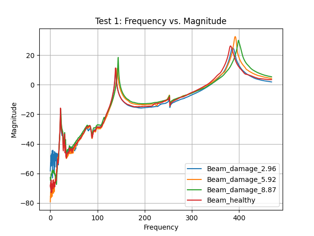
Frequency- Magnitude graph for sample 1 from all 4 classes
After some head-scratching, I plotted the frequency-magnitude graphs for each damage label. I noticed that the first three vibrational modes—around 10–40 Hz, 120–160 Hz, and 350–450 Hz—were crucial for differentiating between healthy and damaged states. Frequencies outside those ranges barely changed with damage.
So, I decided to filter out everything else. The moment I did that, the transformer finally began to learn. It makes sense: the model could now focus on the specific resonant frequencies most affected by mass removal, rather than wasting attention on irrelevant data.
Adding a Little Convolution
I also tested a hybrid CNN + Transformer approach. Convolutional layers are great at extracting local patterns—like those resonance peaks—while reducing the overall sequence length. Feeding these more compact features into the transformer gave a modest performance boost, but it wasn’t the magic bullet. The real breakthrough came from more direct tuning of the transformer itself.
Tweaking Hyperparameters and Batch Size
Increasing the Depth
I increased the number of encoder layers from 2 to 3. This gave the model more capacity to capture the nuanced relationships in the frequency data, especially now that it was focusing on the most important frequency bands.
Reducing the Batch Size
I was initially using batch_size = 8. Training accuracy would shoot up, but validation accuracy wouldn’t budge—or sometimes even dropped. Out of curiosity, I reduced the batch size to 4, then to 2. This slower, more frequent update cycle allowed the model to generalize better, especially given our small dataset of just 280 samples total.
In one experiment, I noticed that with batch_size = 4, the model improved steadily across epochs, rather than jumping around. When I took it even lower, to batch_size = 2, it finally converged to an accuracy I was really happy with.
Final Results
Putting it all together—filtering to critical frequency bands, adding a third transformer layer, and dropping batch_size to 2—yielded an awesome test accuracy of 0.9786. Below is the classification report in a clearer table form:
| Class | Precision | Recall | F1-Score | Support |
|---|---|---|---|---|
| Healthy | 0.99 | 0.94 | 0.96 | 70 |
| Damage 2.96 | 0.95 | 0.99 | 0.97 | 70 |
| Damage 5.92 | 1.00 | 0.99 | 0.99 | 70 |
| Damage 8.87 | 0.99 | 1.00 | 0.99 | 70 |
| Accuracy | – | – | 0.98 | 280 |
| Macro Avg | 0.98 | 0.98 | 0.98 | 280 |
| Weighted Avg | 0.98 | 0.98 | 0.98 | 280 |
And here’s the confusion matrix:
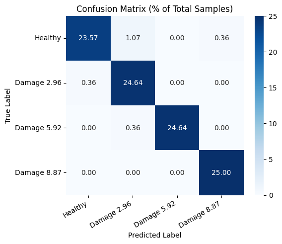
Confusion Matrix: Transformer Model on Beam-Signal Dataset
As you can see, each damage class is identified with very high precision and recall, making this model a solid choice for real-time structural health monitoring.
Wrapping Up
So, that’s the story of how a simple transformer model went from 25% accuracy to nearly 98% on a relatively small dataset:
- We focused on the most relevant frequency bands (the first three vibrational modes).
- We tuned the transformer (adding layers and adjusting batch size) to handle limited data.
- We confirmed that domain knowledge—like knowing which frequencies matter most—is as crucial as model architecture.
If you’re thinking of applying a similar approach, remember that transformers can be quite data-hungry. Whenever possible, gather more data or use strategies like data augmentation. But if that’s not feasible, zero in on the parts of your signal that truly matter. The combination of domain insight and careful hyperparameter tuning can go a long way in bridging the gap.
Thanks for reading this entire series! I hope it’s been helpful for anyone diving into structural health monitoring or exploring how transformers can be adapted to time/frequency-domain data. If you have any questions or want to share your own experiences, feel free to leave a comment or reach out.
Happy modeling!