
Transformer based Structural Health Monitoring using Frequency Response Function (FRF) - Part 3
Published:
Dataset Contents and Structure
The dataset contains 280 samples, with 70 samples for each damage condition, providing balanced data for machine learning analysis. Each sample consists of a 6400-point frequency spectrum stored as numerical arrays in MATLAB (.mat) files within zip archives.
The files provided are:
| File Name | Size | Description |
|---|---|---|
| Dataset Beam-signal_Damaged-5.92.zip | 5.0 MB | Frequency domain data for Damaged-5.92% condition |
| Dataset Beam-signal_Damaged-8.87.zip | 5.0 MB | Frequency domain data for Damaged-8.87% condition |
| Dataset Beam-signal_Healthy.zip | 5.0 MB | Frequency domain data for Healthy condition |
| Dateset Beam-signal_Damaged-2.96.zip | 5.0 MB | Frequency domain data for Damaged-2.96% condition |
| DI_FRAC_Exp-estimation.xlsx | 15.5 kB | Experimental damage index estimations |
| Mass position.xlsx | 119.5 kB | Positions of masses on the beam |
| Beam_Reinforced_Masses.png | 165.7 kB | Image of beam setup with masses |
| BeamMasses.png | 100.9 kB | Additional image of beam setup |
The zip files contain the primary vibration data, while the Excel files offer supporting information. “DI_FRAC_Exp-estimation.xlsx” contains damage indices calculated from frequency response functions to measure damage severity. “Mass position.xlsx” specifies how masses are arranged on the beam, helping understand the damage simulation process.
Two images—”Beam_Reinforced_Masses.png” and “BeamMasses.png”—show the experimental setup, displaying the beam and its attached masses to provide visual context.
Data Format and Accessibility
Each frequency spectrum represents an inertance response in the frequency domain, expressed as magnitude and phase or real and imaginary components. The file sizes (5.0 MB per zip) align with the expected storage requirements for 70 samples per condition, with each sample containing 6400 data points stored as floating-point numbers.
The dataset is freely available on Zenodo, where users can download individual files or the complete archive. Its DOI (10.5281/zenodo.8081690) enables proper citation, and Zenodo’s DataCite integration supports academic indexing.
In this dataset, the Frequency Response Assurance Criterion (FRAC) is used to compute a damage index (DI) by comparing the frequency response functions (FRFs) of a beam under healthy and damaged conditions. The experimental protocol induces damage by removing reinforcement masses (producing mass loss levels of 2.96%, 5.92%, and 8.87%), which in turn alters the beam’s vibrational characteristics.
The computed DI values are then organized into two clustered components, DI-1 and DI-2. Although both indices originate from the FRAC method, clustering them into two groups helps capture different aspects or features of the damage effect on the structure.
FRAC Principle:The FRAC method involves correlating the entire FRF spectrum of a damaged beam with that of a reference (healthy) beam.
- A high correlation (values close to 1) indicates that the dynamic response of the beam is similar to the healthy condition, meaning little or no damage.
- A low correlation (values approaching 0) suggests significant deviation from the healthy state, reflecting damage severity.
- Computation Process:
- The FRF (both magnitude and phase) is measured for the beam under different health conditions.
- The FRAC is calculated (often over specific frequency bands most sensitive to damage) by comparing the measured response against a baseline healthy response.
- The resulting damage index is a normalized value between 0 and 1.
This process is detailed in Sousa et al. (2023), where the authors show that the DI decreases as damage (mass loss) increases, thereby quantifying the severity of the damage
Limitation of Having Only Frequency Domain Signal in Terms of Real-Time Structural Analysis Using AI
While our previous posts have focused on analyzing the frequency-domain representation of the vibration data, relying solely on this information comes with some limitations for real-time structural health monitoring. In this section, we’ll discuss why converting time-domain signals into richer time-frequency representations is beneficial, and how techniques like the Short-Time Fourier Transform (STFT) can bridge the gap.
Why Pure Frequency Domain Data Falls Short
When we analyze a signal in the frequency domain, we typically obtain a static picture that summarizes the overall frequency content of the vibration. Although this provides useful information about the beam’s dynamic characteristics, it does not capture how these frequencies evolve over time. This temporal evolution is crucial for real-time monitoring because:
- Transient Events: Sudden changes or transient phenomena—such as abrupt impacts or evolving damage—may be smoothed out in a pure frequency-domain view.
- Dynamic Behavior: Structural responses can vary with time due to operational or environmental factors. A static frequency spectrum may not capture these variations, limiting the effectiveness of damage detection in real time.
Converting to a Richer Time-Frequency Representation
To overcome these limitations, we can use the Short-Time Fourier Transform (STFT). The STFT divides the signal into short segments (or windows) and computes the Fourier Transform on each, resulting in a two-dimensional representation that shows how the signal’s frequency content changes over time.
A Simple Look at the Short-Time Fourier Transform (STFT)
If you’d like a quick, intuitive explanation of how the Short-Time Fourier Transform (STFT) works, check out this helpful video (specifically from 1:20 to 3:49).
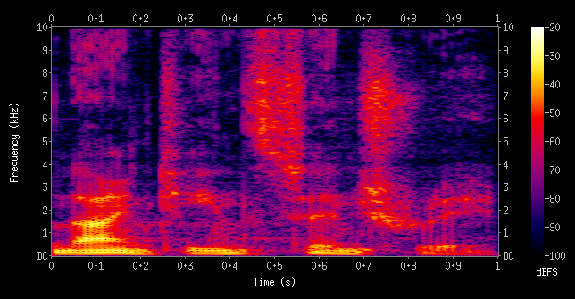
A spectrogram visualizing the results of a STFT of the words "nineteenth century". Here, frequencies are shown increasing up the vertical axis, and time on the horizontal axis. The legend to the right shows that the color intensity increases with the density
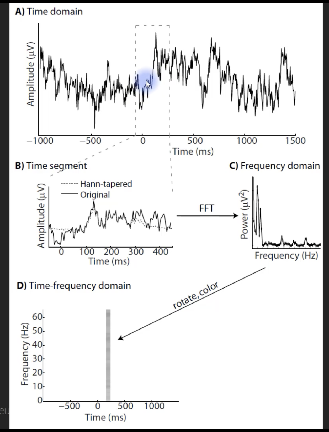
From time-domain graph -> time segment -> frequency-domain graph -> time frequency domain graph
Here’s a brief summary of the concept shown in the image above:
Time-Domain Signal (A)
We start with a vibration signal in the time domain, think of it as amplitude plotted against time.Segmenting the Signal (B)
Instead of taking the entire signal at once, we select a short window of data. This window can be tapered (for example, using a Hann window) to reduce edge effects.Fourier Transform on Each Segment (C)
We apply the Fourier Transform to each short segment. This gives us a snapshot of the frequency content for that specific time slice.Building the Time-Frequency View (D)
By sliding the window along the signal (one segment after another) and performing the transform repeatedly, we end up with multiple frequency snapshots. When we arrange these snapshots in chronological order, we get a spectrogram—a time-frequency representation where:- The x-axis is time.
- The y-axis is frequency.
- The color intensity (or third dimension) represents amplitude.
Time-Frequency Representation for AI and Real-Time Monitoring
Once vibration data has been converted to a time-frequency representation—for instance, using the Short-Time Fourier Transform (STFT)—it becomes far more valuable for AI-based structural health monitoring. Here are the key reasons why:
Dense and Informative Representation
By plotting frequency content against time, the STFT produces a spectrogram that resembles an image. Each “pixel” corresponds to a specific frequency at a specific moment, with color intensity (or height) indicating amplitude. This granular view makes it easier to spot subtle changes or emerging patterns that might be missed in a single frequency-domain snapshot.Leveraging Transformer Models
Transformer architectures have excelled in tasks that require capturing both local and global patterns, from natural language processing to computer vision. When fed with spectrograms, transformers can analyze complex sequences of data—identifying transient damage signatures, tracking how frequencies shift over time, and learning from even small anomalies. This leads to more robust damage detection and prognosis.Real-Time Inference on Edge Devices
One of the greatest strengths of time-frequency data is its applicability to real-time monitoring. After training on spectrograms, AI models—particularly those based on transformers—can be compressed or optimized for edge devices. This enables near-instant detection of anomalies or damage progression, even in resource-constrained environments like remote monitoring stations or onboard sensors.Enhanced Damage Detection and Prognosis
With the STFT, sudden or transient events (e.g., impacts, fast-developing cracks) become more visible as they appear in the time-frequency map. Detecting these events quickly is crucial for preventing further damage and ensuring safety. The detailed view also helps with prognosis, allowing operators to estimate how a fault might evolve under continued stress.
Putting It All Together
While the frequency-domain data discussed in Part 1 and Part 2 provides essential insights, it alone cannot capture the temporal evolution of vibrations. By incorporating a time-frequency approach such as the STFT, you gain a richer perspective that is especially useful for transformer-based AI models. These models can be deployed for real-time structural health monitoring on edge devices, enabling proactive maintenance decisions and helping to prevent catastrophic failures.
Whether you’re a vibration engineer or an AI practitioner, understanding how to leverage time-frequency data for structural health monitoring can significantly improve damage detection and reduce downtime—ultimately leading to safer and more efficient structures.