
Transformer based Structural Health Monitoring using Frequency Response Function (FRF) - Part 2
Published:
Why Convert Time-Domain Data to the Frequency Domain?
In Part 1 of this series, we introduced the beam-signal dataset and showed how vibrations were measured using an accelerometer. We also included graphs illustrating how the beam’s acceleration changes over time (time-domain signals) and mentioned that our dataset primarily consists of frequency-domain data.
You might be wondering why the time-domain signals are converted into frequency-domain representations in the given dataset. In this post, we’ll explore the importance of frequency-domain analysis in structural health monitoring. We’ll revisit some of the concepts from the first post, explain the advantages of working in the frequency domain, and highlight how this representation can reveal critical details about the beam’s behavior that may be harder to see in time-domain signals alone.
Referring to Images and Graphs from Part 1
If you’d like a refresher on the time-domain graphs, take a look at the “Vibration Visualization” section in Part 1. Those images illustrate the beam’s motion over time. In this post, we’ll focus on how that same motion looks in the frequency domain and discuss why this perspective is so useful for detecting and analyzing damage.
Understanding Frequency-Domain Analysis
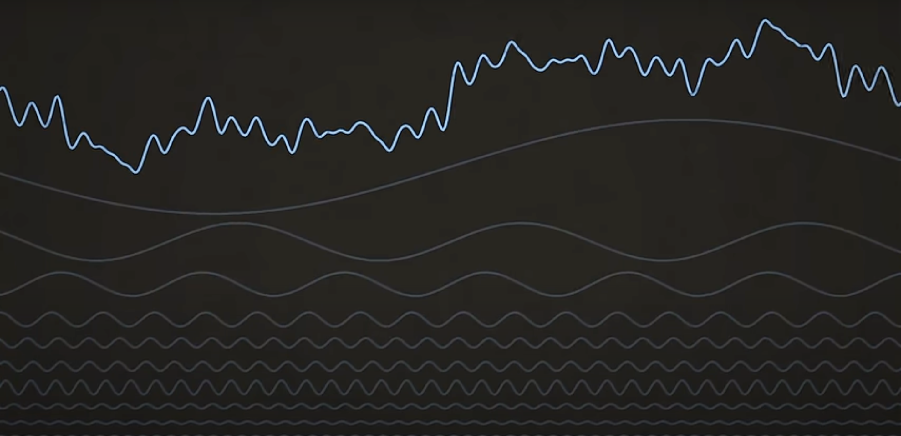
The time-domain signal, illustrated by the left acceleration-to-time graph in the part-1 is complex. If you examine it closely, you’ll notice that the acceleration doesn’t settle into constant upper and lower bounds like a perfect sinusoidal wave. Instead, it varies with each cycle, suggesting an underlying pattern. In reality, the signal is a combination of multiple sinusoidal waveforms superimposed on one another.
To understand this, in simple terms, we can see that the motor at the one end of the cantilever beam is exciting the beam. If you zoom in to the motor. The motor will usually rotate and it will be converted to translation motion (up and down acceleration) by connecting some mechanism to it. In our case there are multiple weights attached to the beam. So imagine one vibration exciting another vibration (like rotating motor to translating acceleration, then it induces vibration in every masses attached to the cantilever beam one by one. Every single vibration has it’s own frequency and amplitude. Why is it so ? In simple terms while transfering one energy (vibration) from one medium to another medium some energy got lost and the vibration pattern varies. But thechnically there are multiple factors involved here like reflection, attuniation, and scattering or distortion.
So at the accelerometer, all this individual sinusoidal wave patterns were combined and create a complex pattern of vibration. So now our job is to untangle them into individual wave patterns. That is what is done above that from time-domain graph to frequency - magnitude(Inertance) graph.
How it is done ?
It is done using the method called Fast Fourier Transform (FFT).
Here we will first look at the brute force method of how time-domain signal is converted to frequency-domain signal.
If you want to know how much of a particular sin wave is in a signal, just multiply the signal by the sin wave at each point and then add up the area under the curve.
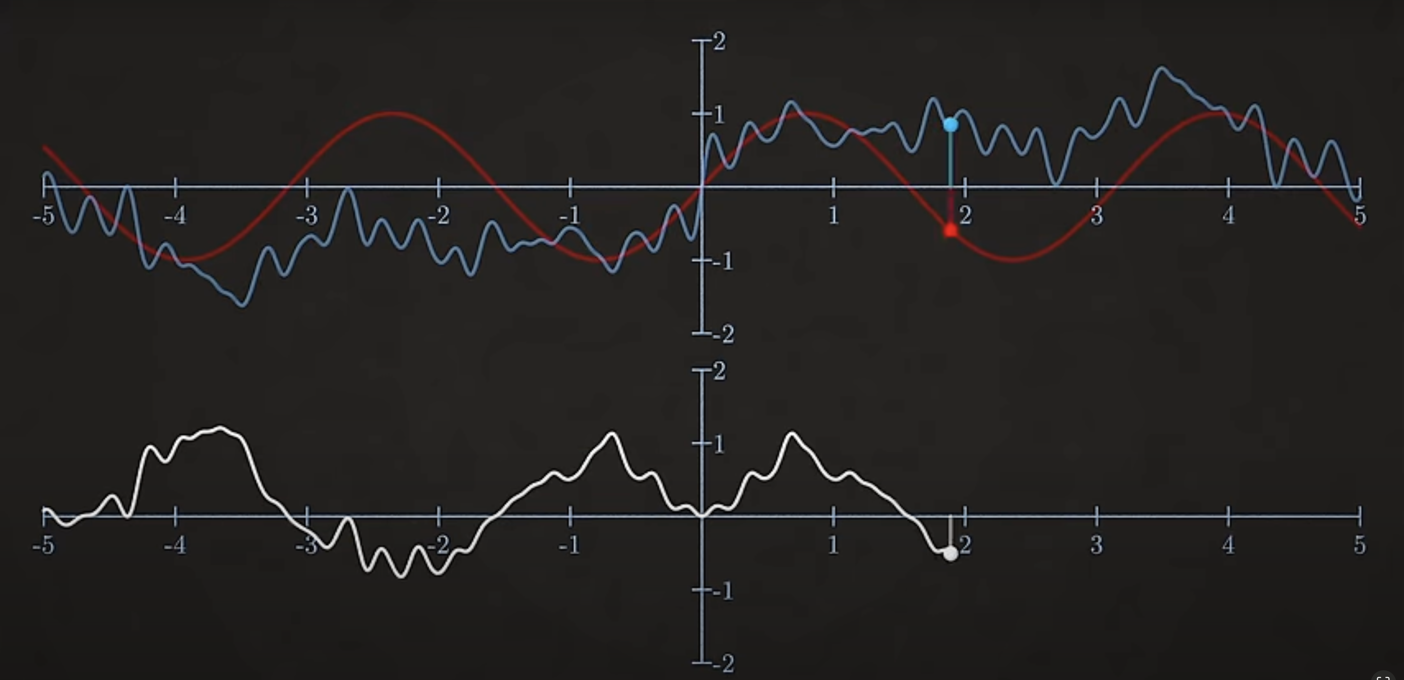
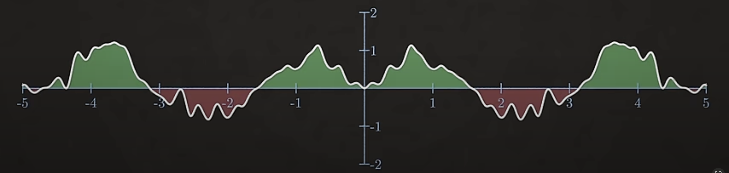
As a simple example, say our signal is just a sin wave with a certain frequency, then pretend we dont know that. And we try to figure out which sin waves add to make it up, if you multiply the signal with a sin wave of arbirtary frequency. The wave are uncorrelated. Means you are just as likely to find places where they upto same both positive or both negative as they were have opposite sign, and therfore when you multiply them together the area above the x axis is equal to the area below the x axis, so these areas add up to zero, which means that frequency sine waves is not part of your signal.
The sine wave and vibration wave are uncorellated (i,e) at some places both positive or both negative (multiplied to get magnitude in positive direction)
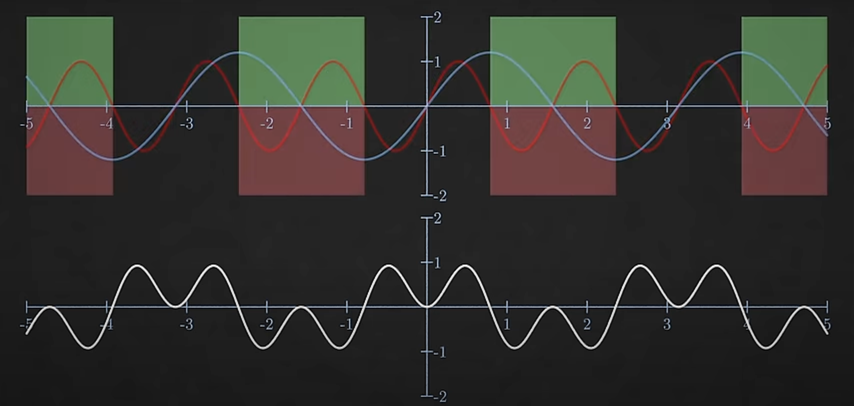
The sine wave and vibration wave are uncorellated (i,e) at some places they are opposite to each other (multiplied to get magnitude in negative direction)
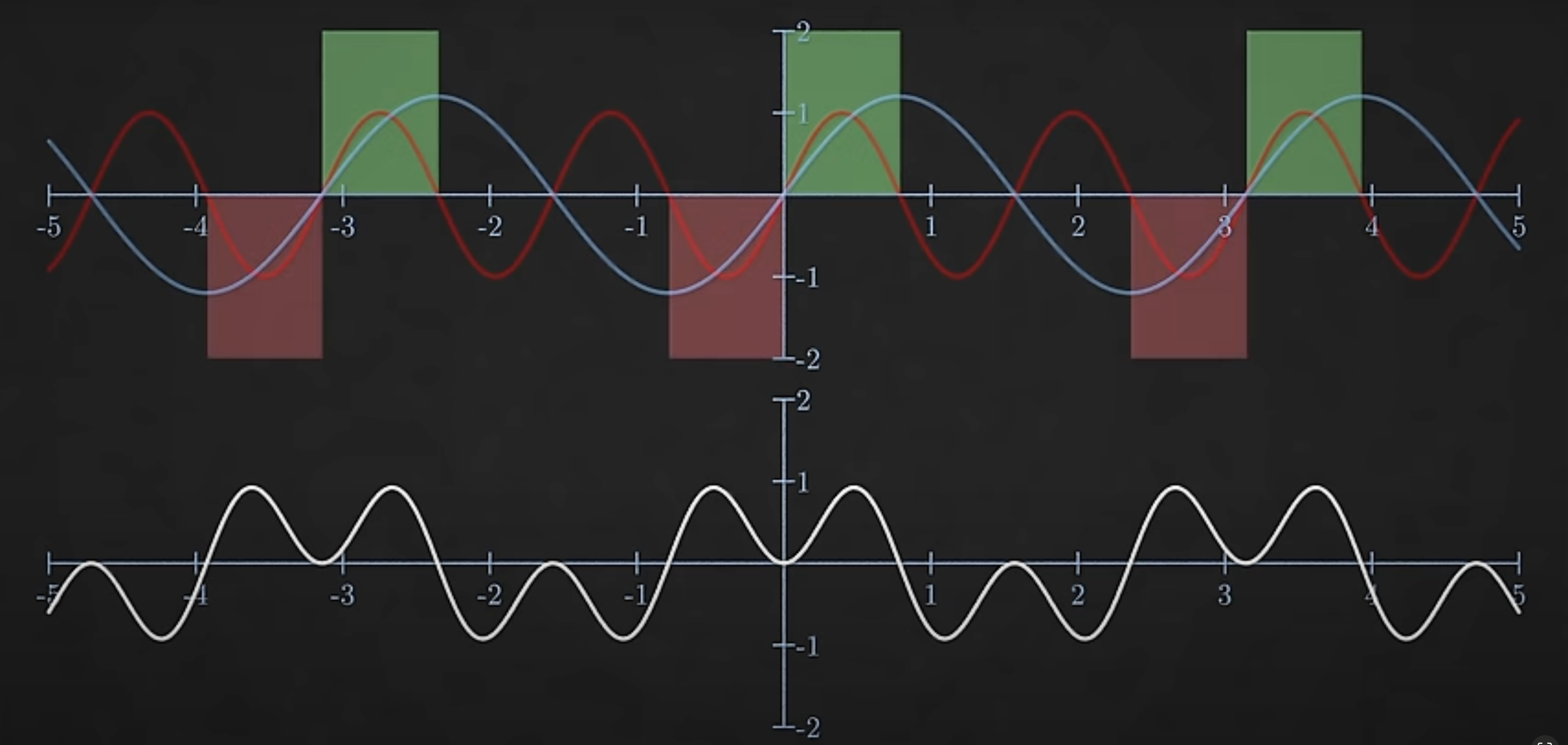
And this will be true for almost all frequencies you could try (assuming we are looking over a long enough time frame), the only exception is if the frequency of the sine wave exactly matches that of the signal. Now these waves are corelated, so their product is always positive so is the area under the curve. That indicated that this sine wave is part of our signal.
And the same trick works even if the signal is composed of bunch of different frequencies. If the sin waves frequency is one of the components of the signal it will correlate with the signal producing a non zero area.And the size of the area tells you the relative amplitude of that frequency sin wave in the signal.
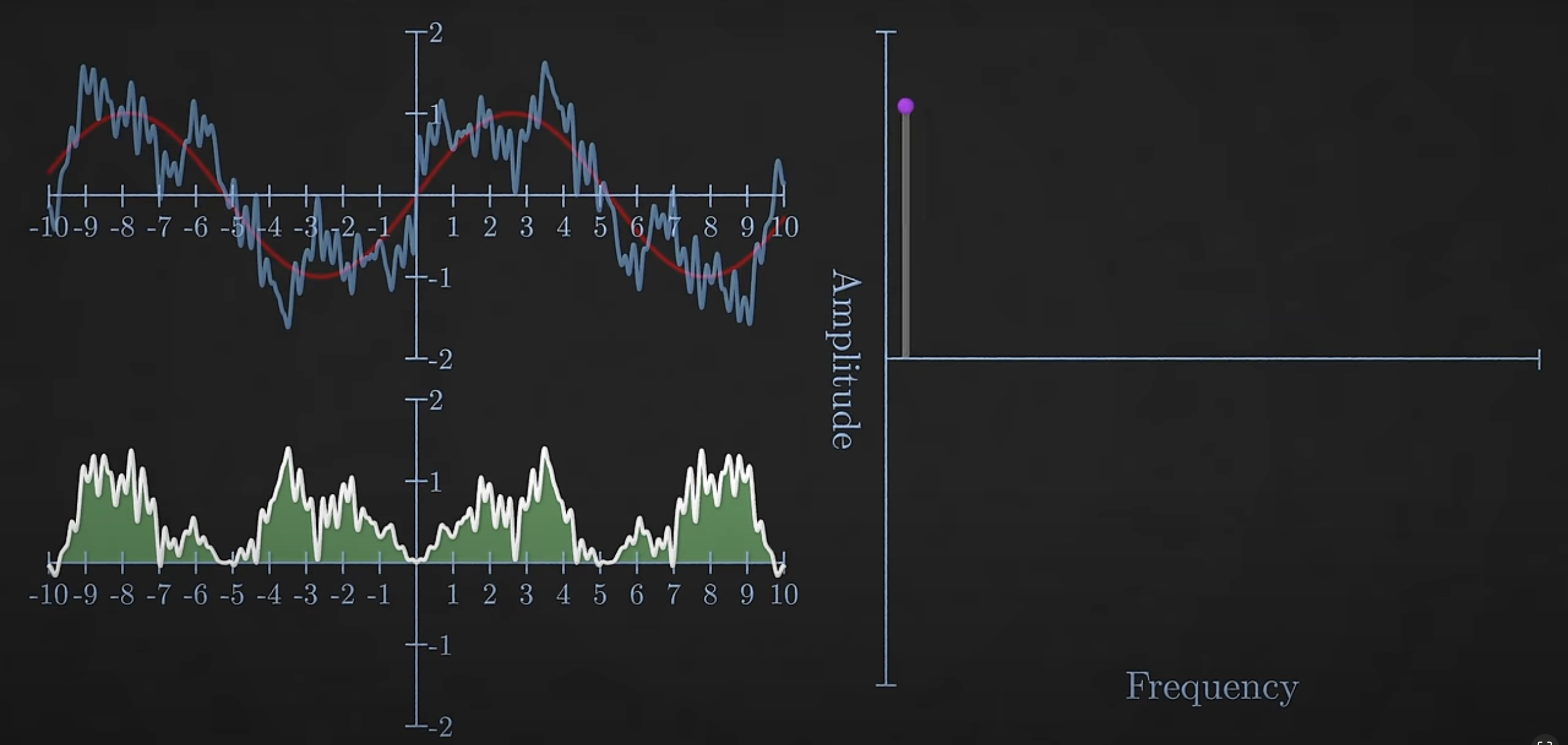
Sum of Area under curve for a signle wave signal makes up an Amplitude value for a frequency in frequency-amplitude graph
Repeat this process for all frequencies of sin wave and you get the frequency spectrum, essentially which frequencies are present and in what proportions.
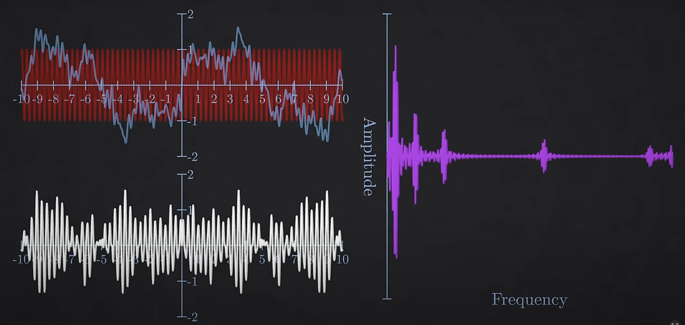
Similarly, multiple sine wave with different frequencies multiplication fills up the frequency-amplitude graph
So far we have only talked about sin wave, but if the signal is a cosine wave then even if you multiply a sin wave of exact same frequency the area under the curve will add up to zero. So for each frequency we actually need to multiply by a sin wave and cosine wave and find the amplitudes for each , the ratio of these amplitides indicates the phase of the signal ( that is how much it is shifted to the left or right). You can calculate the sin and cosine amplitudes seperately or you can use Euler’s formula, so you only need to multiply your signal by one exponent term.
\[e^{j 2\pi f t} = \cos(2\pi f t) + j \sin(2\pi f t)\]Using the above eqn will make the process easy, as the magnitutde is average of cosine and sin wave amplitudes (square root of sum of squares of real(cosine) and imaginary(sine) part $\sqrt{\cos^2 \theta + \sin^2 \theta}$), whereas phase value is the tan inverse of imaginary part divided by real part ( theta from the eqn , $\tan \theta = \frac{\sin \theta}{\cos \theta}$).
Okay! here we are seeing the Amplitude - frequency graph. But actually it is Inertance- frequency graph.
What is Inertance?
Inertance is a type of frequency response function (FRF) commonly used in vibration analysis. It describes how a structure (in this case, a beam) accelerates in response to an applied force across a range of frequencies. Mathematically, inertance A(f) at a frequency f is defined as:
\(A(f)= Force(f)/Acceleration(f)\) The accelerometer records a time‐domain signal. Applying a Fourier Transform (typically via the Fast Fourier Transform, FFT) converts this signal into a complex frequency spectrum. Consider the Fast Fourier Transform is doing the same brute force method with very less conmputation to be performed.
Complex Representation:
Each frequency component is represented as a complex number,
\[A(f) = \text{Re}\{A(f)\} + j \,\text{Im}\{A(f)\} X(f) = \text{Re}\{A(f)\} + j \,\text{Im}\{A(f)\}\]Magnitude and Phase:
- The magnitude is given by \(|A(f)| = \sqrt{\text{Re}\{A(f)\}^2 + \text{Im}\{A(f)\}^2}\)
- The phase is the angle of this complex number: \(\text{Phase}(f) = \arctan\left(\frac{\text{Im}\{A(f)\}}{\text{Re}\{A(f)\}}\right)\)
Now let’s come the dataset, the dataset contais the 0-2000 Hz, 6400 points, 0.3125 Hz discretisation, measured with a PCB 353B03 accelerometer and Polytec VibSoft-20 system. what does this mean ?
The real world data is not continueous, the accelerometer will collect data with a constant interval, in this case it is 6400 points of measurement of accelerometer for every experiment. Converting the accelerometer data (acceleration-time graph) to Magnitude -Frequency domain will also contain the same number of bins of frequency. Why so ? because we can map more number of frequency to a less number of measurement points of accelerometer data.
Example below, there are 8 number of amplitude-time graph. We will first fit it with 1 frequency sin wave, then 2,3,4 .. 8. After that we cannot try to fit 9 frequency signal to 8 data points as it is pointless. So we can calculate only 8 frequency values (instead of single value here it consists of range of value for every frequency bin F0, F1, .. F7).
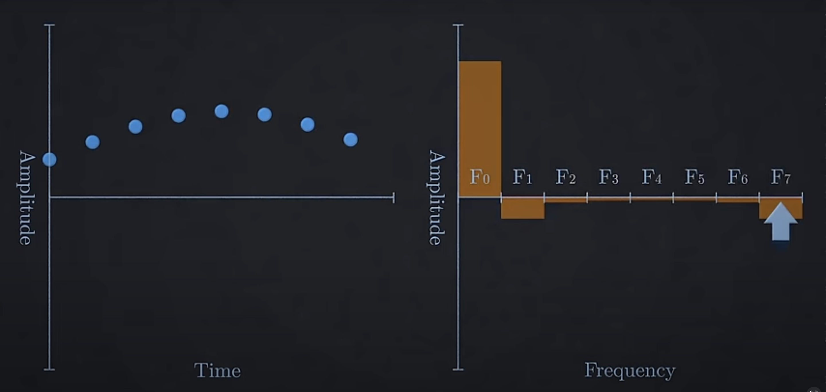
So since we took acceleration measurement of 6400 data points in acceleration-time signal, we convert it into 6400 frequency bins with each bin ranges to distance of 0.3125 Hz added to total 0-2000 Hz frequency range ( (2000 - 0) / (6400 - 1) ≈ 0.3125 Hz) .