
Transformer based Structural Health Monitoring using Frequency Response Function (FRF) - Part 1
Published:
Table of Contents
- Introduction
- How the Damage is Shown
- Does It Perfectly-Represent Real Damage?
- Dataset Background
- Vibration Measurements
- Vibration Visualization
Introduction
This multi-part blog post explores structural health monitoring and structural analysis methods applied to a publicly available dataset. The dataset named beam-signal, it features frequency-domain vibration signals recorded from a beam reinforced with masses, under both healthy and faulty conditions (Zenodo Record 8081690).
We will employ deep learning techniques to analyze the data. This dataset supports research in damage detection, uncertainty quantification, stochastic modeling, and more. However, before diving into the analysis, it’s essential to develop a deep understanding of the dataset itself. In this section, I’ll provide a comprehensive background that even readers with basic mathematical knowledge can follow. Initially, I debated whether to jump straight into the results or build a strong foundation first, I chose the latter, aiming to address every question an average reader might have.
For more details on the project, you can also check out the project repository.
Let’s begin!
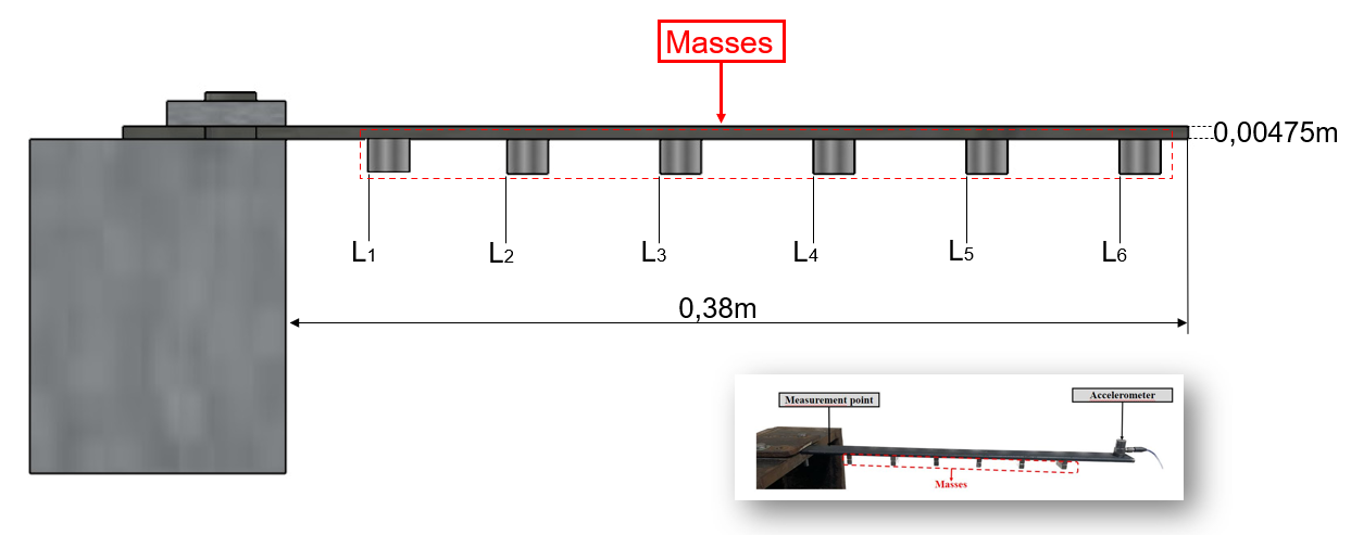
The above image shows the experimental setup used to collect the dataset.
Dataset Background
The dataset, published on November 8, 2023, is an open-access resource contributed by the University of Brasília and Bydgoszcz University of Science and Technology. It is part of a broader effort to advance research in structural health monitoring (SHM), particularly through the analysis of vibration data from a physical beam under various damage conditions. Its availability on Zenodo (Zenodo Record 8081690) ensures accessibility for the research community, with a DOI for citation and integration into scholarly workflows.
The primary purpose of the dataset is to facilitate damage assessment of a beam reinforced with masses, simulating different levels of structural integrity. Damage is induced by altering the mass distribution through the removal of mass blocks (as shown above), which leads to varying degrees of mass loss:
How the Damage is Shown
In this experiment, instead of inducing actual structural damage (such as cracks or material degradation), damage is simulated by selectively removing small masses from the beam. The beam is initially equipped with several small weights. For instance, if the beam starts with 100 grams of extra weights, then:
- Removing 2.96 grams simulates the lightest damage.
- Removing 5.92 grams represents moderate damage.
- Removing 8.87 grams corresponds to the most significant simulated damage.
For each of these conditions, including the healthy state (with no mass removed), 70 samples were collected. This controlled removal of mass offers a precise way to mimic changes in the beam’s vibrational behavior, enabling a systematic study of damage effects.
Does It Perfectly Represent Real Damage?
Not perfectly, but it’s a good approximation. In the real world, damage might be in the form of a crack, rust, or a hole—things that alter the beam’s strength and weight. Removing masses mimics this by reducing its weight and changing its vibration characteristics, much like a crack would. The percentages (2.96%, 5.92%, 8.87%) help precisely control and measure the “damage” in this experiment, making it useful to study.
Vibration Measurements
The beam undergoes vibration, and the vibration signals are measured in the frequency domain as inertance responses, which relate force to acceleration. Each spectrum spans a frequency range from 0 to 2000 Hz, with 6400 points and a resolution of approximately 0.3125 Hz calculated as:
\(\frac{2000 - 0}{6400 - 1} \approx 0.3125 \text{ Hz}\)
Let’s break down this concept for those not familiar with the scientific terminology. While the description may seem simple, understanding it requires some knowledge of mathematics and structural vibrations. Let’s go through these concepts one by one.
Vibration Visualization
Watch the Vibration Video
This video demonstrates the vibration of a cantilever beam. When you measure the vibration at a specific point on the beam over time, you can plot a graph of acceleration versus time.
Imagine the free end of the beam:
- It starts at the center of the flat section.
- It moves upward, decelerating until it reaches the topmost point, where it momentarily stops.
- Then it accelerates downward until it reaches the center again.
- This cycle repeats, with deceleration as it approaches the bottommost point.
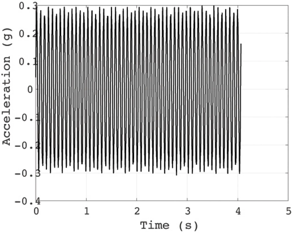
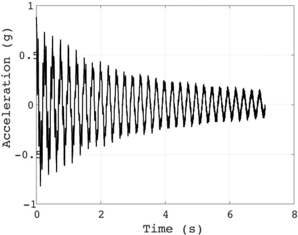
The right graph below represents the signal measured during free vibration of the structure, while the left graph shows the signal when the structure is under steady-state excitation, resulting in a nearly constant acceleration graph.
Signal measured in the free-vibration of the structure using the ADXL-335 accelerometer
Signal measured when the structure is excited by a frequency of 13.12 Hz using the ADXL-335 accelerometer
However, the dataset does not include these time-domain graphs. Instead, it provides the processed data in the frequency domain.
Below are the frequency domain graphs corresponding to the above signals:
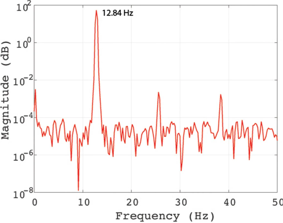
Signal measured in the free-vibration of the structure using the ADXL-335 accelerometer (Power Spectrum Density)
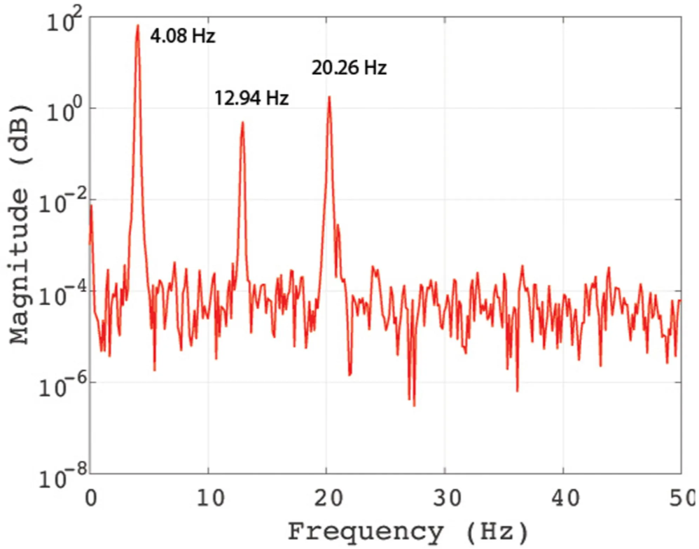
Signal measured in the free-vibration of the structure using the ADXL-335 accelerometer (Power Spectrum Density)